Through in-context learning, transformer models can prove effective for classifying tabular data.
German university researchers had demonstrated this in 2023 under the TabPFN banner. By 2025, they broadened the scope to include regression.
The same year saw the emergence of an open model adopting the in-context learning approach: TabICL (ICL for “in-context learning”). It widened the learning window to up to 500,000 examples, thanks to an architecture called “column-then-row.” Broadly speaking, it involves a three-stage pipeline, with attention applied successively to columns, then rows, then the entire dataset.
The v2, released in 2026, boosted performance, notably by integrating the Muon optimizer and a query-aware scalable softmax.
One model, one pretraining phase
H2O.ai reused this architecture to design its own tabular foundation model: TabH2O. After presenting it in mid-April, it leveraged Dell Technologies World (May 18–21) to showcase it again.
From one month to the next, the pitch remained the same: advantageous compared to traditional ML because no per-dataset tuning is required. Also advantageous compared to AutoML because it consumes fewer resources. And advantageous compared to TabICL due to several architectural evolutions.
First, classification and regression are handled by a single model, with two heads. Each mini-batch of pretraining paired datasets covering one and the other task (80% and 20%, respectively). This mechanism helped reduce resource consumption.
Another difference that further reduced the footprint: pretraining is in a single phase. With TabICL, it required three (500,000 steps, then 40,000, then 10,000) due to stability concerns. Techniques such as RMSNorm normalization and logit capping reinforced this stability, allowing the model to start working on sequences of maximum length right away (12,288 rows with up to 100 features). In the end, around 6.4 million synthetic datasets were needed, whereas TabICL v2 used nearly 35 million.
“Up to 500,000 rows per GPU”
To create a synthetic dataset, a random DAG is sampled (edge density configurable; up to 10 parents per node). Each node is assigned a function type (among 8), and root values are sampled from several distributions and propagated through the DAG.
On large datasets, TabH2O can fragment the processing. It splits the training rows into sub-batches and averages the predictions. In combination with the key-value cache and activation offloading, this enables up to 500,000 rows per GPU.
H2O.ai offers the model via its API, with the following limits in the free version:
- 2 requests per minute
- 20 requests per day
- 500 requests per month
- 100,000 rows per request
- 100 columns
Clustering and missing-value imputation are paid features. Excel and Google Sheets plugins are available, as well as a skill for agents. Regression on time series remains experimental. And multimodality is currently out of scope.
Less resource-hungry than TabICL, but less performant
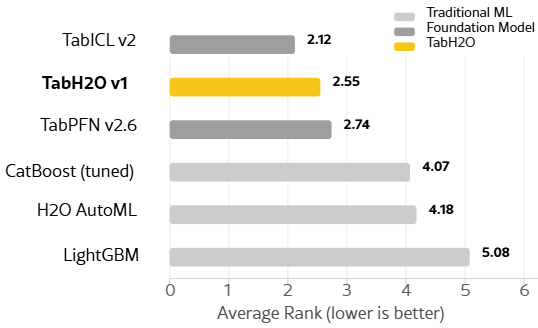
In April, H2O.ai reported some performance scores on the TALENT benchmark (300 datasets). Without getting into the evaluation details, it announced an average score of 2.37 (the lower, the better). That placed TabH2O between TabPFN and TabICL. It added that, on average, one could expect:
- 1.1 seconds to process 1,500 rows
- 1.4 seconds for 7,000 rows
- 2.9 seconds for 15,000 rows
- About 20 seconds for 50,000 rows
The score announced at Dell Technologies World is somewhat lower (2.55). But the same goes for the other models. H2O.ai is only marginally more precise on its testing methodology (three tasks, six methods). It emphasizes a metric intended to reflect real-world usage: regardless of the number of columns, predictions arrive in under 3 seconds for datasets up to 10,000 rows.
On smaller datasets, the network is the main source of latency. For 1,000 rows and 20 columns, inference sits at 189 ms, versus a 0.4 s round-trip API. With the largest configuration tested (500,000 rows by 50 features), prediction arrives in about 5 minutes with fragmented processing.